Automatic tracking
The intended workflow is as follows:
Obtain nucleus positions.
Obtain division likelihoods.
Obtain link likelihoods.
Create tracks (i.e., possible lineages made of probable links)
Calculate error probabilities.
Manually correct warnings to improve tracks.
OR Do automated analysis only with best tracks.
Before you start, create a directory that will hold all the results of your analysis (e.g., automated_tracking inside the directory that holds your images).
Step 1: Obtain nucleus positions
Open the OrganoidTracker GUI and load your images (File -> Load images...). For the best results, the input data should somewhat resemble the training data. This can often be achieved with a little pre-processing (See here for tips).
Select Tools -> Peform automatic cell tracking.... OrganoidTracker will switch to a window dedicated for automatic cell tracker. The File/Edit/View-menu at the top has now changed: there should now be a Parameters and a Cell tracking menu. Use the Parameters -> Set positions model folder... mnu option. You will be prompted to select the neural network trained for detecting nuclear positions. (See here for how to train a model or find links to pre-trained models at our Github page.)
In the Cell tracking menu, select Preview position detection to see how well the selected model performs on your data. If the preview looks bad, proceed to the ‘Troubleshooting’ section below. Once the nucleus position detection looks OK, proceed to Cell tracking -> Predict positions in all time points.... A dialog box will prompt you to create a folder for storing the detected positions by typing the new folder’s name (e.g., positions within automated_tracking).
You now have a folder (e.g. positions) containing configuration files and scripts with the name organoid_tracker_predict_positions. To run the script, double-click the BAT file (Windows) or the SH file (Linux). If it crashes with an out-of-memory error, try closing other programs (including the OrganoidTracker GUI) and try again.
After running the script, you have a folder called Automatic positions that contains a .aut file with a name like the input image you are analyzing. You can load this .aut file (File->Load tracking data... or simply drag in the file) alongside the microscopy image to assess the quality of the predictions.
If you want to debug this step, open the organoid_tracker.ini file and give the predictions_output_folder setting a value, for example test. If you run the script again, it will create a folder with that name (test in this example) and place images there indicating how likely it is to find a cell there.
Troubleshooting
If the predicted positions do not look good, there are some options available in OrganoidTracker GUI to improve the results:
Make sure the right channel is selected for nucleus detection in the
Parameters->Set image channel for prediction...menu. You can also select multiple channels, which will be summed before passing them to the neural network.If the model randomly predictions positions in the background, increase the value of
Parameters->Set min intensity quantile...to perform intensity rescaling.If your nuclei have varying intensity, and only the brightest nuclei are detected, decrease the value of
Parameters->Set max intensity quantile...to make the brightest nuclei less bright in comparison to the rest.If the resolution of your images is different from the training data, or your nuclei are simply particularly large or small, you can rescale the images before passing them to the neural network. Use
Parameters->Set XY scaling...orParameters->Set Z scaling...to do this.
Correcting for changed image offsets
When taking longer time lapse movies, the organoid can slowly slide out of the view. For this reason, the microscope user can move the imaged area so that the organoid stays in the view. In the time lapse movie, this makes the organoid appear to “teleport”: from the edges of the image it jumps back to the center.
To create links over this “jump”, the program would need to create a lot of large-distance links. The program will likely refuse to do this. To correct for this, before running the linking process, open the OrganoidTracker GUI and load the images and positions (File menu). Then edit the data (Edit -> Manually change data...) and edit the image offsets (Edit -> Edit image offsets...) of the correct time point. Instructions are on the bottom of the window.
Step 2: Obtain division likelihoods
With both the images and nuclear positions loaded into the OrganoidTracker GUI, again go to Tools -> Peform automatic cell tracking..., then use Parameters -> Set divisions model folder. When prompted by the dialog box, select the neural network trained for detecting cell divisions. Then, you can optionally preview the division predictions in the Cell tracking menu, and then run the division predictions for all time points using Cell tracking -> Predict divisions in all time points. You will be prompted to create a folder for storing the detected divisions by typing its name (e.g., divisions within automated_tracking). As with step 1, this will generate various files and folders. Run the organoid_tracker_predict_divisions script.
After the script is finished, you have a folder called Division predictions containing a new .aut file also named after the microscopy image. Use File->Load tracking data... to visualize the results alongside the original microscopy image.
If you double-click on a cell in the main window, you can view its data, which now includes the division probability. Verify that this probability is what you would expect: high for cells that are about to divide, low otherwise.
Step 3: Obtaining link likelihoods
With both the images and divisions loaded into the OrganoidTracker GUI, select Tools -> Peform automatic cell tracking... and then Parameters -> Set links model folder. When prompted by the dialog box, select the neural network trained for detecting links (i.e., connections between the same nucleus in consecutive timepoints). Next, optionally preview the links and then use Cell tracking -> Predict links in all time points. This will prompt you to create a folder for storing the links by typing its name (e.g., links within automated_tracking). As with step 1, this will generate various files and folders. Run the organoid_tracker_predict_links script.
After the script is finished, you have a folder called Link predictions containing a new .aut file also named after the microscopy image. This contains all links that OrganoidTracker considers to be possible (e.g. links to the nearest position, plus links to positions at most two times as far as the nearest position). Use File->Load tracking data... to visualize the results alongside the original microscopy image.
Step 4: Create tracks
With both the images and links loaded into the OrganoidTracker GUI, select Tools -> Peform automatic cell tracking... and then Cell tracking -> Create tracks.... You will also be prompted to create a folder for storing the tracks by typing its name (e.g., tracks within automated_tracking). As with step 1, this will generate various files and folders. Run the organoid_tracker_create_tracks script.
This will generate a folder called Output tracks, which contains a folder with the same name as the original microscopy image. Within that folder there are four .aut files. As indicated by the name, these contain either All possible links (useful for calculating error rates) or a most probable subset (Final links). These exist as two versions, clean or raw.
Now you can also set some parameters to clean up the data after tracking. It is advisable to at least remove very short tracks for clarity.
Troubleshooting
You can modify this step of the analysis by changing the following values in the configuration file (e.g., organoid_tracker.ini within tracks).
maximum z depth for which we want tracks: 22 (pixels, default) Remove tracks that start or end above this pixel height, as “deeper” slices are noisier and harder to segment and therefore track. Consider decreasing this value to focus on higher quality segmentations when creating tracks.margin_um: 8 (μm, default) Defines a margin at the image edge; positions within that margin have higher probabilities to disappear and appear. Consider increasing this margin if cells move a lot.min appearance probability: 0.01 (default) False negative rate of cell detection. This value need not be exact to get good performance as it does not substantially affect results. Can be affected by cells “appearing” from outside the field of view, but themargin_umparameter (see above) already accounts for this by automatically increasing probabilites of appearance within a defined border region.min disappearance probability: 0.01 (default) False negative rate of cell detection plus the death rate of cells. Consider adjusting to match the known death rate, but this value need not be exact to get good performance. Can be affected by cells “disappearing” to outside the field of view, but themargin_umparameter (see above) accounts for this by automatically increasing probabilites of disappearance within a defined border region.
Step 5: Calculate error rates
With both the images and Final links - clean.aut loaded into the OrganoidTracker GUI, select Tools -> Compute marginalized error rates.... When prompted, select the all possible links file (All possible links - clean.aut) and then create a folder for storing the output (e.g., error_rates). Run the resulting organoid_tracker_marginalization script.
This should be produce a file called Filtered positions.aut.
Troubleshooting
You can modify this step of the analysis by changing the following values in the configuration file (e.g., organoid_tracker.ini within error_rates).
maximum error rate: 0.01 (default) Links with marginal probability < (1-maximum error rate) are removed (e.g, links must exceed threshold probability of 0.99 for the default value of 0.01). Consider adjusting this value to make the threshold more or less stringent.temperature (to account for shared information): 1.5 (default) Scales probabilities before calculating marginalized probabilites across all possible states; in this way, accounts for shared information between neural network predictions and can absorb miscalibrations of the neural network outputs. Nonetheless, needs to be calibrated to each model. If your data are sufficiently similar to the intestinal organoid data we trained our models on, you can use the default value. Otherwise, calibrate yourself.
Step 6: Manually correct warnings
This step is not automated. 😉
With both the images and Filtered positions.aut loaded into the OrganoidTracker GUI, go to Edit -> Manually change data.... A cross will appear over all locations where the program has detected some inconsistency in the tracking data:
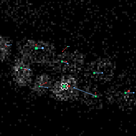
To view why OrganoidTracker warned you about this position, hover you mouse over a nucleus and press E. This will show you what the warning is. If the warning was a false positive, just press Delete to delete the warning. Otherwise, exit the warning screen (press E or Escape). This takes you back to the cell track editor, where you can fix the error.
To fix errors, you can edit the data using mainly the Insert and Delete keys, which are used to insert and delete links (respectively). Detected positions can also be inserted and deleted if necessary. Because correcting data works exactly the same as manual tracking, please see the manual tracking tutorial for more information.
If you press Left and Right in the warning screen, you will be taken to other warnings in the same lineage. If you press Up or Down, you will be taken to the warnings of other lineage trees.
If you press the L key from the cell track editor, a screen is opened that shows whether there are still warnings remaining in the lineage of that cell. If you hover your mouse over such a lineage and press E, the program will take you to the (first) warning in that lineage tree.
If you don’t want to correct everything, there are several options:
Limiting the number of time steps that you are looking at. In the warning screen, if you open the Edit menu, there’s an option to set the minimum and maximum time point for correction.
Limiting the area you are looking at. This is most easily done by pressing L in the cell track editor, and then observing any lineages that still have warnings. Correct any lineages that need to be corrected (press E while you hover your mouse over them). Once you are satisfied, you can then delete all lineages that still have errors in them. This is done from the cell track editor: press
Edit > Batch deletion > Delete lineages with errors. See batch editing for more ways to delete a lot of lineages at once.
You can change a few settings of the error checker, to make it stricter or less strict. In the error checking screen (the screen you opened with E) there are three options available in the Edit menu: the minimimum marginalized probability a link should have, the minimum time in between two cell divisions of the same cell, and the maximum distance a cell may move per minute (only useful before marginalization).
Often correcting mistakes below a certain threshold also fixes a few mistakes that were not flagged. The increase in tracking quality might therefore be more than naively expected. To check the resulting quality you can rerun the marginalization on your corrected data while flagging in the organoid_tracker.ini file that you have checked part or all of the errors.
What to do if I have too many errors to correct?
That’s a difficult problem! You have a few options:
Improve image quality. The images should be good enough that it is straightforward to track the nuclei by hand in the large majority of cases.
Change some settings. See the earlier troubleshooting steps. In addition, the generated
organoid_tracker.inicontain additional settings, with an explanation for each of the settings.
Step 7: Automated analysis
In step 5 a set of filtered high-confidence tracks is produced. You can choose to analyze these further. Generally for many application, manual corrections are not needed.
If you want to quantify a fluorescence reporter you can take long tracks (
Edit->Manually change data->Batch deletion->Delete short lineages) and work from there.If you want to quantify tissue flows flawless trajectories are often overkill. Setting a lower probability threshold should still give you good enough data.
Analyzing cell cycle dynamics should be done using survival analysis (See here for how to do this) anyway and this can deal with cells that are lost to follow up. So it is not a problem to use the uncorrected filtered data.